Musical Analysis of Rush Part 1: Musical Development Over Time
Introduction
In our previous post, we downloaded the relevant data and munged it into tibbles
thanks to the wonderful spotifyr package.
In this initial analysis notebook, we want to analyze Rush’s musical history over time. We will do
this using Spotify’s audio API ggplot2, the ggrepel addon. Spotify’s audio features that we use here are as follows. Any feature with a * next to it is one that we are not using.
| Feature | Description |
|---|---|
| acousticness | A confidence measure from 0.0 to 1.0 of whether the track is acoustic. 1.0 represents high confidence the track is acoustic. |
| danceability | Danceability describes how suitable a track is for dancing based on a combination of musical elements including tempo, rhythm stability, beat strength, and overall regularity. A value of 0.0 is least danceable and 1.0 is most danceable. |
| energy | Energy is a measure from 0.0 to 1.0 and represents a perceptual measure of intensity and activity. Typically, energetic tracks feel fast, loud, and noisy. For example, death metal has high energy, while a Bach prelude scores low on the scale. Perceptual features contributing to this attribute include dynamic range, perceived loudness, timbre, onset rate, and general entropy. |
| instrumentalness | Predicts whether a track contains no vocals. “Ooh” and “aah” sounds are treated as instrumental in this context. Rap or spoken word tracks are clearly “vocal”. The closer the instrumentalness value is to 1.0, the greater likelihood the track contains no vocal content. Values above 0.5 are intended to represent instrumental tracks, but confidence is higher as the value approaches 1.0. |
| liveness* | Detects the presence of an audience in the recording. Higher liveness values represent an increased probability that the track was performed live. A value above 0.8 provides strong likelihood that the track is live. |
| loudness* | The overall loudness of a track in decibels (dB). Loudness values are averaged across the entire track and are useful for comparing relative loudness of tracks. Loudness is the quality of a sound that is the primary psychological correlate of physical strength (amplitude). Values typical range between -60 and 0 db. |
| speechiness | Speechiness detects the presence of spoken words in a track. The more exclusively speech-like the recording (e.g. talk show, audio book, poetry), the closer to 1.0 the attribute value. Values above 0.66 describe tracks that are probably made entirely of spoken words. Values between 0.33 and 0.66 describe tracks that may contain both music and speech, either in sections or layered, including such cases as rap music. Values below 0.33 most likely represent music and other non-speech-like tracks. |
| tempo | The overall estimated tempo of a track in beats per minute (BPM). In musical terminology, tempo is the speed or pace of a given piece and derives directly from the average beat duration. |
| valence | A measure from 0.0 to 1.0 describing the musical positiveness conveyed by a track. Tracks with high valence sound more positive (e.g. happy, cheerful, euphoric), while tracks with low valence sound more negative (e.g. sad, depressed, angry). |
## Necessary to load fonts properly
library(dplyr)
library(readr)
library(here)

## Packages for plotting
library(ggplot2)
library(ggrepel)
library(extrafont)

source(here("lib", "vars.R"))

rush_albums <- readRDS(RUSH_ALBUMS)
Let’s plot each variable over time. To do this, we need to first gather all of the musical feature columns. Then we’ll make a facetted plot.
There’s one issue though, which is that we have 165 tracks. That’s a lot of dots for a time series! We’ll calculate a weighted average of each of these variables at the album level. The weighting will be by track duration because Rush has many long songs that dominate most of an album. The title track of 2112, which is 20 minutes long, should not be weighted the same as A Passage to Bangkok, which is 3 minutes long.
Since we currently have each musical feature in its own column, let’s make a tidy tibble consisting
of one musical feature per row. This will allow us to use facet_wrap when building our plot to
have one feature per facet. To make our plot prettier, we’ll also change feature names to begin
with capital letters.
library(tidyr)

album_duration_dat <- rush_albums %>%
    group_by(album_name) %>%
    summarize(album_duration_ms = sum(duration_ms))

album_stats <- rush_albums %>%
    group_by(album_name) %>%
    gather(feature, value,
           danceability, energy, acousticness, instrumentalness, valence, tempo) %>%
    inner_join(album_duration_dat, by = "album_name") %>%
    mutate(track_weight = duration_ms / album_duration_ms,  ## Generate weighted features
           weighted_value = track_weight * value) %>%
    group_by(album_name, album_release_date, feature) %>%
    summarize(value = mean(value),
              weighted_value = sum(weighted_value)) %>%
    ungroup() %>%
    mutate(feature = Hmisc::capitalize(feature)) %>% ## acousticness -> Acousticness
    arrange(album_release_date)
Plotting the Data
We will be using some helpful packages to make our plots look nice. They are:
ggrepel: Lets us make labels and text boxes that automatically dodge each other. We have a lot of labels, so this will prevent our charts from being piles of illegible text.extrafont: Lets us load non-default fonts. I’m using the Working Man font from the RUSH Font Project.
rush_plot <- album_stats %>%
    rename(Feature = feature) %>%
    ggplot(aes(x = album_release_date, y = weighted_value, label = album_name)) +
    geom_line(aes(color = Feature)) +
    geom_label_repel(alpha = 0.6, size = 2) +
    facet_wrap(~ Feature, scales = "free", ncol = 1, nrow = 6) +
    labs(title = "Musical development of Rush over time") +
    theme(plot.title = element_text(family = "Working Man", size = 22),
          legend.position = "none") +
    xlab("Release Date") +
    ylab("Value")
plot(rush_plot)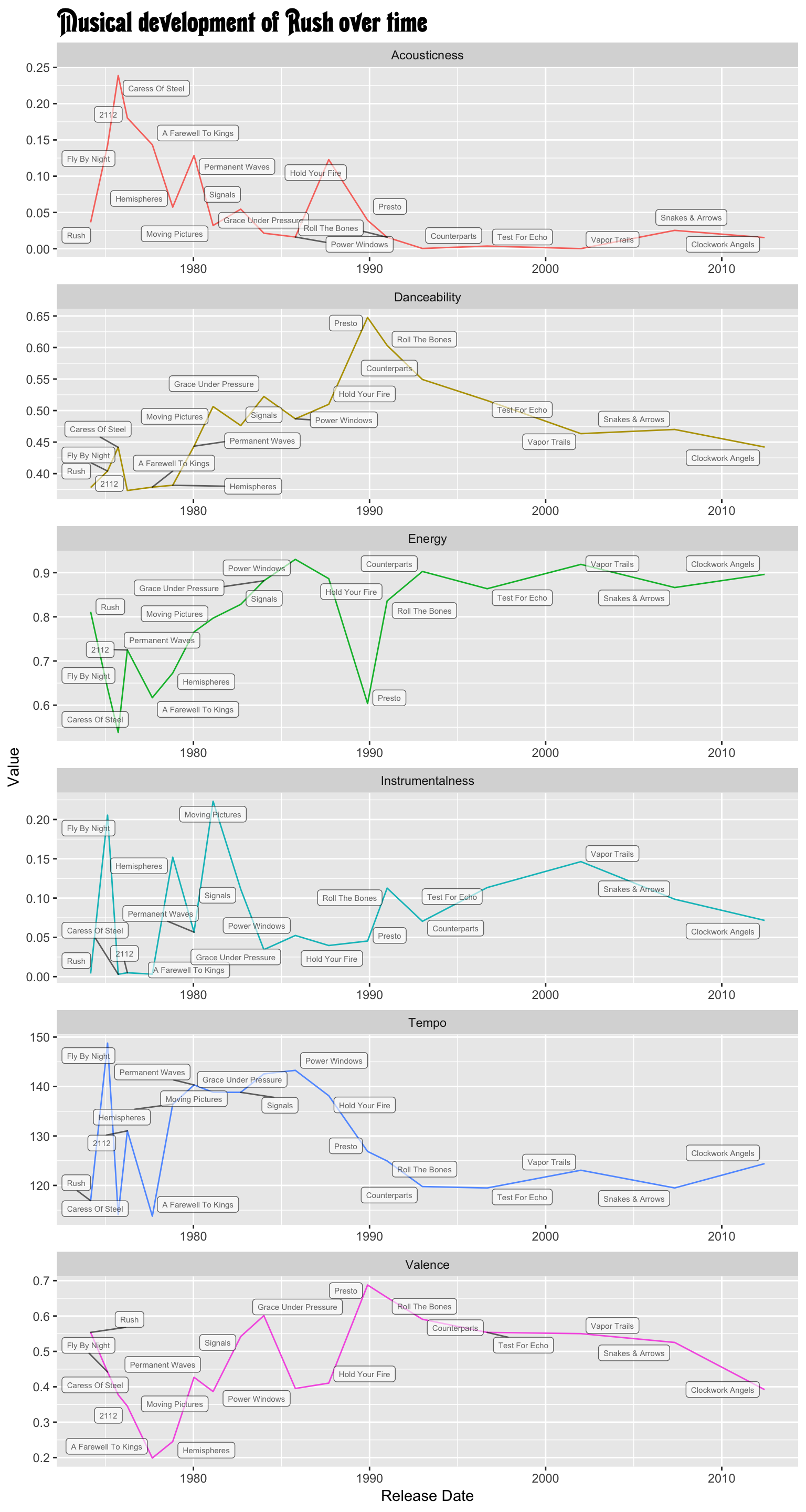
Here’s what we see:
Moving Pictures is not only the most instrumental Rush album, but it marks a peak at which Rush’s music got less instrumental. As they added more synthesizers to fit in with their 80s contemporaries, Rush also added more vocals to the mix. However Rush has never been in danger of becoming an instrumental band, as we see no “Instrumentalness” values above 0.2
For reference, the highest possible “Instrumentalness” value is 1.Caress of Steel is Rush’s most acoustic album, and also has among the lowest danceability and energy scores.
Power Windows, which is dominated by synthesizers and fast tracks, has high energy and low acousticness.
Rush’s music has gotten slower over time. It’s interesting how after Power Windows, when Rush decided that they didn’t want to be a progressive rock band dominated by synthesizers, Rush’s music quickly started dropping in average tempo over the course of their next four albums, reaching 120BPM on Counterparts and staying approximately there until Clockwork Angels.
There is one data point that I am very curious about. Why does Fly By Night have such a high instrumentalness score when all of its tracks have lyrics? Let’s take a look at the individual track values for the album.
rush_albums %>%
    filter(album_name == "Fly By Night") %>%
    select(track_name, instrumentalness, duration_ms)
## # A tibble: 8 x 3
## track_name instrumentalness duration_ms
## <chr> <dbl> <dbl>
## 1 Anthem 0.328 261760
## 2 Best I Can 0.418 205573
## 3 Beneath, Between & Behind 0.000128 181933
## 4 By-Tor And The Snow Dog 0.283 517373
## 5 Fly By Night 0.000994 202200
## 6 Making Memories 0.00529 177707
## 7 Rivendell 0.264 297093
## 8 In The End 0.159 406600My suspicion is that it’s being driven by By-Tor and the Snow Dog, which is the longest track on the album and has long instrumental sections. Similarly, Anthem and Best I Can have lyrics but lean instrumental. Anthem has no vocals until 54 seconds into a four minute song. Best I Can has similar instrumental sections.
Next Steps
Now that we’ve traced Rush’s musical development over time, we’re going to do some clustering next. It’ll be interesting to see what groups of albums hierarchical clustering discovers.
saveRDS(album_stats, ALBUM_STATS)