Musical Analysis of Rush Part 2: Clustering Rush Albums

July 22, 2018 analysis

Now that we’ve looked at Rush’s musical development over time, let’s do some hierarchical clustering based on music features. This is heavily inspired by, if not plagiaried, directly from Alyssa Goldberg’s similar analysis on David Bowie albums.

library(ggplot2)
library(dplyr)
library(tidyr)
library(tibble)
library(here)
library(rpart)
library(dendextend) ## for colors
library(circlize) ## one of the only times where circles are nice
library(spotifyr)

source(here("lib", "vars.R"))

album_stats <- readRDS(ALBUM_STATS)

First of all, our data is in long format where each row is “musical feature of an album”. We need it to be in wide format, where each row is “all musical features for an album”. To do this, let’s use tidyr::spread. After all, it’s the opposite operation of tidyr::gather, which we utilized when prepping this data.

We’ll make two frames: One where the values have been weighted by track length, and another where they haven’t been. Since hclust needs a matrix of values, we’ll also do that transformation here.

Since the process to make both data frames is virtually the same, I’ll write a function that uses dplyr’s new quasiquotation features. I’d like to pass multiple columns for col_to_drop, but sadly this seems like more trouble than it’s worth right now.

One thing to note is that in most cluster analyses, you should center and scale the variables to mean 0 and standard deviation 1 to prevent values that have a larger range from being weighted more. But because all musical features except for tempo are on the same \([0, 1]\) scale except for tempo, we scale tempo to be between \([0, 1]\) to ensure that all features are treated equally during clustering..

prep_df_for_cluster <- function(dat, val_col, col_to_drop) {
    ## Given a data frame, a value column, and a bunch of columns to drop,
    ## return a data.frame appropriate for clustering.

    val_col <- enquo(val_col)
    col_to_drop <- enquo(col_to_drop)
    
    dat %>%
        select(-!!col_to_drop, -album_release_date) %>% 
        spread(feature, !!val_col) %>%
        mutate(Tempo = scales::rescale(Tempo, c(0, 1))) %>% 
        column_to_rownames("album_name") %>%
        as.data.frame()
}    

rush_albums_for_weighted_cluster <- prep_df_for_cluster(album_stats, weighted_value, value)
rush_albums_for_unweighted_cluster <- prep_df_for_cluster(album_stats, value, weighted_value)

Clustering

Now that the data is prepped, let’s do the clustering. Here’s a hierarchical clustering of Rush albums. You should read this as “albums in the same color are in the same cluster.” I picked Ward linkage for the clustering after significant trial and error.

First, let’s cluster the weighted albums.

dend <- as.dendrogram(hclust(dist(rush_albums_for_weighted_cluster), method = "ward.D2")) %>%
    color_branches(k = 4) %>%
    color_labels(k = 4)

circlize_dendrogram(dend, labels_track_height = 0.4, dend_track_height = 0.4)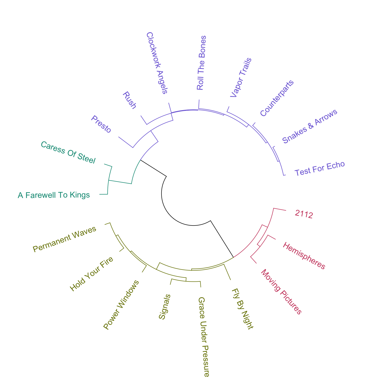

…and then the unweighted albums

unweighted_dend <- as.dendrogram(hclust(dist(rush_albums_for_unweighted_cluster), method = "ward.D2")) %>%
    color_branches(k = 4) %>%
    color_labels(k = 4)

circlize_dendrogram(unweighted_dend, labels_track_height = 0.4, dend_track_height = 0.4)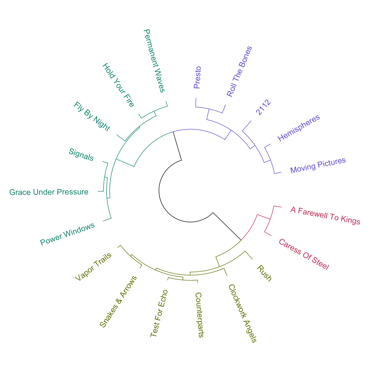

It’s interesting that the clusters for both the weighted and unweighted data look almost identical. I will focus on the weighted clustering because it fits my existing understanding of Rush’s albums.

In the weighted dendrogram, we see the following clusters:

Purple: Hard rock that isn’t heavily experimental. It’s interesting that Rush’s self-titled debut is so similar to their later work like Snakes and Arrows and Clockwork Angels, even though the material in the middle of their career is so different.
Yellow-Green: 80s albums with lots of synthesizers. Fly By Night is in this cluster for unclear reasons, since I suspect it would fit much better with the purple cluster. It looks like a borderline case based on its position in the dendrogram, and because a lot of the clusterings I tested that aren’t displayed here assigned it to seemingly random clusters.
Red: Long compositions with technical and heavily progressive instrumental sections. The three albums in the red cluster are generally considered Rush’s most progressive.
Green: The two albums that came immediately before and after 2112. Both are hard rock and hint at Rush’s future musical development, but are relatively transitional compared to some of the albums in the other clusters.

Fly By Night

Why is Fly By Night in the yellow-green cluster when it is so musically different from the other albums in it? Let’s take a look. What features are most similar between it and the other five albums in its cluster?

yellow_green_albums <- c("Fly By Night", "Grace Under Pressure", "Signals", "Power Windows", "Hold Your Fire", "Permanent Waves")
rush_albums_for_unweighted_cluster[yellow_green_albums, ]

##                      Acousticness Danceability    Energy Instrumentalness
## Fly By Night           0.13873125    0.4401250 0.6645375       0.18230150
## Grace Under Pressure   0.02276612    0.5225000 0.8835000       0.03533150
## Signals                0.06051000    0.4782500 0.8250000       0.12641675
## Power Windows          0.01660475    0.4847500 0.9321250       0.04992494
## Hold Your Fire         0.12939000    0.5077000 0.8826000       0.04045400
## Permanent Waves        0.15103333    0.4793333 0.7478333       0.04485653
##                          Tempo   Valence
## Fly By Night         0.9450388 0.5102500
## Grace Under Pressure 0.9768196 0.6082500
## Signals              0.8879157 0.5516250
## Power Windows        1.0000000 0.3922500
## Hold Your Fire       0.8143972 0.4023000
## Permanent Waves      0.7952627 0.4573333

A quick peek indicates that Fly By Night has really similar danceability, valence, and tempo scores to these other albums. It’s similar in terms of “bounciness”.

Robustness Checking

Now suppose that Rush decided to reunite release a brand new album that’s considerably more poppy and Spanish than what they put out in the past four decades. For the same of argument, let’s call this new track “Despacito”. I’m going to query Despacito, add it to Rush’s discography, and see how it influences the clustering. If these are good clusters, then they should be virtually the same with or without Despacito.

I’ll also do it for Africa by Toto because why not?

library(spotifyr)

get_single_track_features <- function(track_name, slice_num) {
    
    get_tracks(track_name) %>%
        slice(slice_num) %>% 
        get_track_audio_features() %>%
        select(danceability, energy, acousticness, instrumentalness, valence, tempo) %>%
        mutate(album_name = track_name) %>%
        gather(feature, value, acousticness, danceability, energy, instrumentalness, tempo, valence) %>%
        mutate(feature = Hmisc::capitalize(feature)) %>%
        mutate(weighted_value = value)
}    

despacito <- get_single_track_features("Despacito", 2)
africa <- get_single_track_features("Africa", 1) %>% mutate(album_name = "Africa by Toto")


album_stats_with_new_tracks_for_unweighted_clustering <- album_stats %>%  ## Phew!
    bind_rows(africa) %>%
    bind_rows(despacito) %>% 
    prep_df_for_cluster(value, weighted_value)


unweighted_dend_with_new_tracks <- as.dendrogram(hclust(dist(album_stats_with_new_tracks_for_unweighted_clustering), method = "complete")) %>%
    color_branches(k = 6) %>%
    color_labels(k = 6)

circlize_dendrogram(unweighted_dend_with_new_tracks, labels_track_height = 0.4, dend_track_height = 0.4)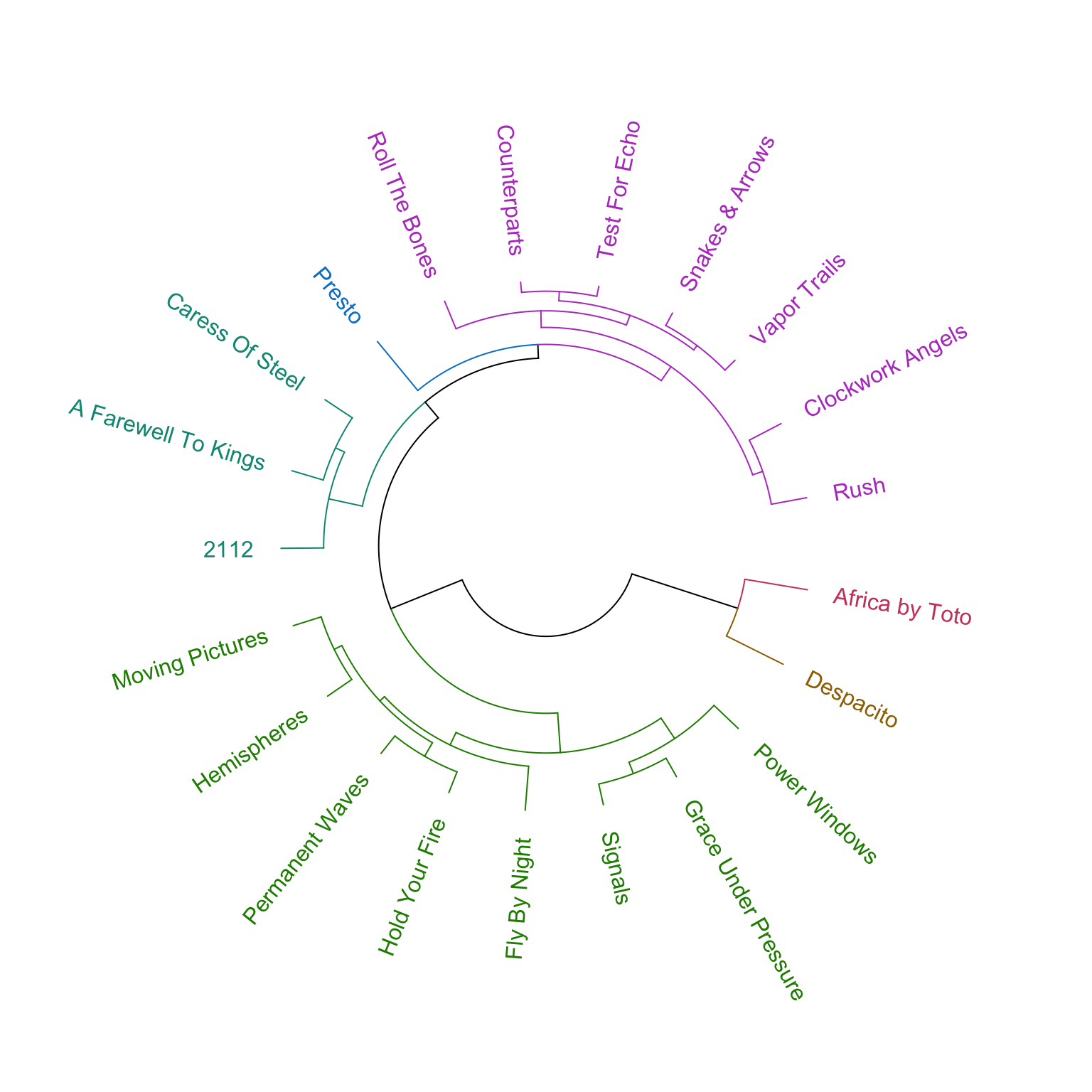

Despacito and Africa are their own cluster. Which makes sense because I’ve never been to a club that played Tom Sawyer by Rush.