Feature Selection with Boruta Part 1: Background and Data Prep
Introduction
Issues with Feature Selection
For the next two posts, I will be exploring the usefulness of the Boruta feature selection algorithm. It is a heuristic algorithm that seeks to find all relevant features, rather than just rank model features in terms of importance. This is useful for two reasons:
- It is rarely the case that some magic number of features predicts the output of interest.
- Feature importances are relative, meaning that even the top four features may not actually be useful in practice.
Imagine we want to identify runners competing in the 100-meter dash at the Olympics who are good. Also suppose we have no idea what the Olympics are, and for all we know, we are looking at 200 random people running.
Selecting good runners under a traditional feature selection scheme would be like saying “give me the ten best runners”. But if there are 200 Olympic runners, all of whom are surely the best runners in their home countries, then the vast majority are amazing runners! Selecting ten runners would mean missing out on a large number of skilled athletes.
\)](/post/boruta/2019-02-03-feature-selection-with-boruta-part-1/2019-02-03-feature-selection-with-boruta-part-1_files/sogelau_400x400.jpg)
Figure 1: Sogelau Tuvalu, a shotputter from American Samoa, entered the 100-meter dash at the 2011 World Championships in Athletics because there were no registration requirements. He finished four seconds behind the second-slowest runner at 15.66 seconds. Presumably, neither feature selection scheme would identify Tuvalu as a great runner. (Source)
How does it work?
This algorithm was originally designed for use with random forests, but can be applied to any type of model that outputs feature importances. In a nutshell, here’s how the algorithm works (explanation taken directly from a talk I gave on this paper in 2016):
At each iteration:
For each feature \(\mathbf{X}_j\), randomly permute it to generate a “shadow feature” (random attribute) \(\mathbf{X}_j^{(s)}\).
Sequentially fit a bunch of random forests on the original and shadow features.
2a. Calculate feature importances on the original and shadow features.
2b. Call the feature “important” for a single run if its importance is higher than that of the maximum importance of all shadow features (MIRA).
Eliminate all features whose importances across all runs are low enough (via a hypothesis test criterion described in the paper). Keep all features whose importances across all runs are high enough. Any feature with importance not sufficiently low or high is “tentatively important”.
Repeat from the beginning with all tentative features until all are declared important or not important, or until a particular number of iterations.
The logic behind Boruta is akin to having a randomly-selected audience member run alongside each runner in the Olympic 100-meter dash. We say that the best runners are those who run faster than the best audience member. Under this criteria, we would say that almost all of the runners are skilled, rather than searching for ten skilled runners.
Use case: Aptamer Detection
I will be replicating the analysis that Kursa, Jankowski, and Rudnicki performed in the original Boruta paper. Their goal is to use Boruta to identify which k-mers are indicative that a given molecule is an aptamer. An aptamer is a class of short DNA or RNA molecules with clinical and research applications. For a given DNA or RNA sequence, a k-mer is a k-letter subsequence1.
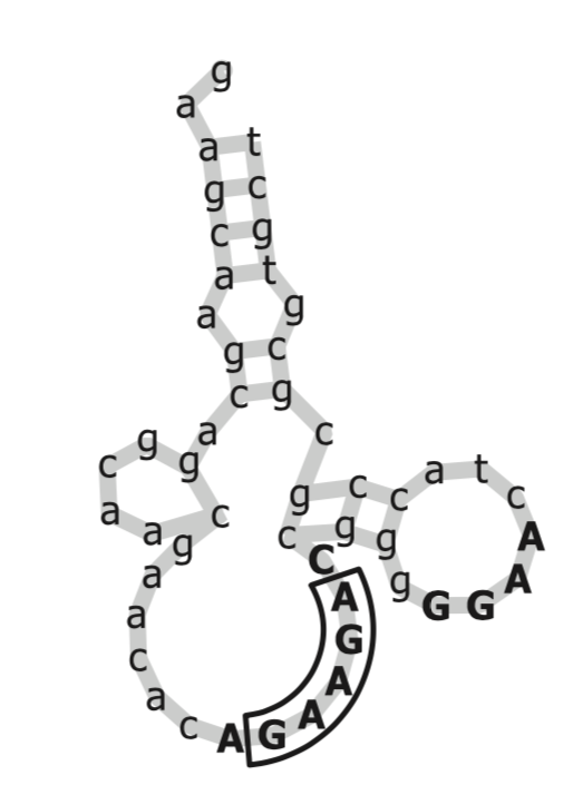
Figure 2: This is an aptamer of ATP, the primary molecule involved in energy production. Boruta found the GGAG 4-mer to be important, while past research indicated that the GAAGA motif was important. (Source is from the original Boruta paper.)
For example, the sequence GAACTAGG contains:
- The 3-mers
GAA,AAC,ACT,CTA,TAG, andAGG. - The 4-mers
GAAC,AACT,CTAG, andTAGG. - The 5-mers
GAACT,AACTA,ACTAG, andCTAGG.
Identifying whether a k-mer marks an aptamer is a difficult problem because each feature is “presence or absence of a 3, 4, or 5-mer.” There is no prior domain knowledge indicating which k-mers are likely to be important, and there are 1344 features2 (columns) with a much smaller number of sequences (rows). Because the authors fit a separate model for each molecule3, and because no molecule in the data has more than 139 aptamer sequences, this is a small \(n\) large \(p\) problem.
Prepping the Data
Before we can start building models, we need to prepare the data. Since the Texas Aptamer website with the data
no longer exists, Miron Kursa sent me a .json file with a bunch of known aptamer sequences for various
models. Here is the data. The authors
generate non-aptamer sequences by permuting the aptamer sequences, which is clever in its
simplicity and because it ensures we have equal numbers of aptamer and non-aptamer sequences, avoiding issues
with imbalanced data.
Let’s take a look at the raw data:
library(jsonlite)
library(tidyverse)
## ── Attaching packages ───────────────────────────────────────────────────────────────────────────────────────────────── tidyverse 1.2.1 ──## ✔ ggplot2 3.1.0 ✔ purrr 0.3.0
## ✔ tibble 2.0.1 ✔ dplyr 0.7.8
## ✔ tidyr 0.8.2 ✔ stringr 1.3.1
## ✔ readr 1.3.1 ✔ forcats 0.3.0## ── Conflicts ──────────────────────────────────────────────────────────────────────────────────────────────────── tidyverse_conflicts() ──
## ✖ dplyr::filter() masks stats::filter()
## ✖ purrr::flatten() masks jsonlite::flatten()
## ✖ dplyr::lag() masks stats::lag()library(rDNAse)
library(here)## here() starts at /Users/brandonsherman/shermstats/content/post/borutalibrary(glue)##
## Attaching package: 'glue'## The following object is masked from 'package:dplyr':
##
## collapselibrary(beepr)
input_file <- here::here("data", "apta-seqs.json")
output_file <- here::here("data", "ATP.rds")
aptamer_json <- fromJSON(input_file)
str(aptamer_json)## List of 23
## $ ATP : chr [1:66] "TCTGTTCTTCAAGGCTGAGATTGCCGTCCGTAATTGAGTGCGGACATGAGAGAGGGTGGA" "GCTGAGGGCCGCGGACGTAATTGCGCGTGGAAGACCCTGCGTGGCCCCTGTTGGATTGT" "TCTGTTGTTAAGGCTGAGATTGCCGTCCGTAATTGAGTGCGGACTAGAGCGGGTAAA" "GGACTTCGGTCCAGTGCTCGTGCACTAGGCCGTTCGACCAGTTGGGAAGAAACTGTGGCACTTCGGTGCCAGCAACTCTTAGACAGGAGGTTAGGTGC" ...
## $ Arginine : chr [1:41] "CCCGTCCGCGGTAGAAAGCCACGTGCACGT" "TCCGTCCGCGGTTGAATTACGAACCACCTA" "GCTTGCGTCGCGGTAGAGCTGATATCTGTG" "AGCGGTTGAGTCCATCTCCGGGCACTGCTC" ...
## $ Codeine : chr [1:47] "CTATAGTGAGGCTATTAAGGGTTGTGGGGG" "TACAGAATAAGCGAATTAAGGGTTGGGGTG" "AAAAGGGTGGTTGAAGGGACAGCTGGTGTG" "AAAAGGGTGGTTGAAGGGACAGCTGGTGTG" ...
## $ Dopamine : chr [1:54] "CTGAAGTCCCGCGTGTGCGCCGCGGGAGACGTTGCAGGATTAATAGCCTCGACGGCGGGTAGATATGTTAGCACATAGTGAGGCGCTGCTCCA" "GGAAGCCGCGTGTGCCCGCCOCGCATCCGACACATTTAAGAATAAGAGCCAGGGTTAAGCAAGCAATGCTGGAGGCAGCTTATTCCGTCA" "CGTTGCACCAGGGTGTAAGGAGGTGACACGTGTCCCAACCTCGATCGAGGAACTCCAACATGTGATACCCGCTCACATAGTTGACG" "AACTCCGCGTGTGCATGGTTAATGGAGTCCTGGGCTCCGGAGAGCACCCGTCGGAGGGTATTTTCTTTAGAATGCTGATACTACCAGCGT" ...
## $ Elastase : chr [1:52] "CAGGAGACGCTACCCACCGGTTACATTGAATATCTCTCCC" "GCCGACGTAGTGTACATTTAAACCAGGGGCCTGCTCTCTA" "CAGCGTCATTTAGGATTCGTCAGGTTCTACCGTAGTGTG" "CGGTGACAACACAGTATCCTATAAAGTCTCACCCTTATGCCA" ...
## $ FAD : chr [1:46] "CGAGAACACATAGCGCTCTTGAACTGCGCGGTCGTGCGCACGCTAATGCTCCTCAGGGATTACAAGAAGGATGCCGGAGT" "GGTCTCACAACACCATGGAGCTACAAGAAAGATGCCATACCAAGGATCCTGTCACACGAAATGTCTGTTCGACAAATGCG" "CAGAAACTTAGACGCAAATACAAAACATCCGGACAACGGCGATTATCGAAGAATGCGGCCTCTTCTCGCGGCCGAGGGTA" "CCAAAACGGGCACTCCCTGATCCAAGAAACAACCGCTAGTTGTCTTTACGTGGAAGACGCAAACTGACCGGTTAGGCTA" ...
## $ HIV1-Tar : chr [1:52] "GGCAGGGTGGAGAGTTACTGGATAGGTATT" "GGCAGGGTGGAGAGTTACTGGATAGGTATT" "CAAGCAGCACATATCTTCTTTACCTTGCC" "CACTGCACTCAACACACTTTCAGTTG" ...
## $ Hematoporphyrin: chr [1:34] "GCGCATTAGGGCGGGTATGGGAGGGGTGGACTGTATGTCAGAGCACGCGAGGGGATGTCTA" "CCAGGGGGAGCCGATGCGGTGTGAGCGAGGAGGGGGTGGTGGGCTATACGATACCGTTTTA" "ACTGGGGATGGGTGGGGAGGGCTGGGATGCAAATTCGGCAGTGGAATCGTGTCAGACTC" "ACTGGGGATGGGTGGGGAGGGCTGGGATGCAAATTCGGCAGTGGAATCGTGTCAGACTC" ...
## $ IDI4 : chr [1:49] "TGTTCTATGGGTGAGTCATACT" "ACTACGAGTCACCATCACGTCC" "ACAATAAATCATCATCCCGCAC" "TATAGGCATTCTTAATAATAGT" ...
## $ Isoleucine : chr [1:139] "TTACGTCCGGAACAAGGACTAGTGGG" "CCGACCGTATGAGAAAGTTGGG" "CTACAGTGCTTTTGNGCGCNCTATTGGG" "TTACGTCATTAGGACTATTGGG" ...
## $ KHdomain : chr [1:33] "AAGAGCTACGCCTGTCCACTCTTGCGCTTC" "CTTACCGACTTTCACTGTGTTACCGCTCT" "TAAACCTCTTTTCTAGCTCCTCTCGCTTA" "TCTGCAGGTAAGTCTAGGTTTTGGTTCTGC" ...
## $ MBGT : chr [1:32] "GGGTAAGGAAGAACCTGTGGCACTTCGGCGCCAAAAACTC" "GGTAGCGGAAGAAACTTTGACACTTCGGTACCAGCAACCC" "GGGAAGGGAAGAATTTGTGACACATCGGTGCCTGCGTCCC" "AGGTAGGGAAGAAAGTGTGGCACCTTCGAGTCAGCAACCC" ...
## $ MS2-cp : chr [1:82] "TGTTGAGTCTGGGGACATGAATACCCAAG" "CACAGGGGGATTGCTTCCTCTATACGGTCC" "CACTCATTTTCATACCATGAGTATGACGNG" "CACTCGAACTCGCGTTTCGAGTATGACGGG" ...
## $ NPY : chr [1:31] "GGGCGCAGACGAAGGGAGGACCTGCATTCATTAAAAACTG" "ATTCAAGGGTAACACATCCAGGGGAACGGAATTGCAGCCC" "TCATCAGTGGAAGGGGCCACAACTCGCTTTGTAGAGTTGG" "GACCGCGCGAGAAAAGGGTTCGTTCGTGAGGAGCGAGAGA" ...
## $ NTS-1 : chr [1:30] "GAAAAGTGAGTAAAAGGGGCCCCTGAACCTCCCGGTGCC" "GGAAAAGATGATATGGGCCCCTGAAAGTCCACCCGGCGCT" "CCGACCTCCATGGAAACATTCTGCGACTACTTACTGGTC" "GCGACTCCTGTACTCGAAGACAGACAGTTCCAGCCTCCAG" ...
## $ REL-GATA : chr [1:125] "CTGGGGGAATTCGAT" "ATGAAGTGGGGACTCACTTGCCCCC" "CTTGGGGGGAATTCTGCAG" "AAATGGGAACCCCCATCCGTACCCA" ...
## $ Sa-methionine : chr [1:34] "TGACGGACCCGATCGTCCAGCGATGATCTGGTGGAAGAATCTGCGTCA" "ACTGGGGCTTTTGCTAAAGTCGGAAGAAAATGCAGT" "GTGTGGAAGATCCTGCGCATGGC" "CGCCAGAACGGACCATGGTGGTAGAAACTGCGTCCTGTG" ...
## $ VEGF165 : chr [1:44] "TAACCGAATTGAAGTTATTGGACGCTACCT" "TAGGAAGAATTGGAAGCGCATTTTCCTCG" "TCAGGAACGGAATTTTTGGAGACACGCCCT" "ATCAGTGAATGCTTATAGACCGCCTCCGT" ...
## $ WT-suppresor : chr [1:30] "CCTTAGAATGATGCGACATG" "ATCACCCACCCCGAGCTGGC" "GATATGGTAGCGCCCGCACG" "CTCCCAACTGACTGACCTGGCGC" ...
## $ g5p : chr [1:32] "GCCGCCACTTCCTCTGGTTTGGTCCC" "CCGCAGCTACATCCTCATGATCCCTT" "CACTCGCGGCCATGCTTATTGATCCC" "CATCCACTCCTTCCATCGGGTCCCGC" ...
## $ hnRNP : chr [1:108] "ACACAGCATAACATATACAC" "ATGTAATTGTTCTCCGCGCA" "ATTACACCACACCCACTCGG" "CCGGACAAACACACGAACAC" ...
## $ pefloxacin : chr [1:42] "CAGGCTGCAGATGCTCACTTTAACGTTGAGATTGGCCGTC" "AAGGCTAGACTGCTAAGAGCGGAGTACCGTCATTGGTGTC" "ATTATACTCATTTCCACTTAGTGGAGAGTCTGGTGAGATC" "GGAGAGACCACTTGAAAAAACAAGGTCGGTTATGTTTAGT" ...
## $ vasopressin : chr [1:43] "CCCGACGTGAATGATAGACGTTACGTGTGTACACGAAGTCGAGTTGCTGTGTGCCGATGAAAGTGGGA" "GATAACGTGATGGATAGACGTAGGGTGTATACACTAAGTCGAGTTGCTGTGTGCCGCTGAACGTGTGA" "ACTGTCGTGAATGATAGACGGTAGGATTATACACTCTGTCGAGATGCTGTGTGCCGATGAACGACGGT" "GAGAGGGTGAATGATAGGCATGACGTGTATACTGTATGCCGAGTTGCTGTGTGCCGATGAACCTCGTA" ...The data consists of molecules as list element names, and aptamer sequences as values in a Python dict-like structure.
The rest of this file will detail the processing of the data into a form useful for analysis.
Here’s the process:
Turn the
listof sequences and aptamers into adata.framefor easy processing.Shuffle the molecules to make non-aptamer sequences.
For each aptamer and non-aptamer sequence:
3a. Generate all possible k-mers of length 3, 4, and 5. The
kmerfunction in therDNAsepackage will handle this.3b. Mark the presence and absence of every one of the 1344 k-mers for the given molecule.
Walkthrough
First, let’s turn the aptamer data into a tidy data.frame. In other words, each
row should be a single observation.
We first turn the json into a nested tibble, then unnest the result.
unprocessed_aptamer_dat <- tibble(molecule = names(aptamer_json),
                   sequence = aptamer_json) %>%
  unnest()

unprocessed_aptamer_dat %>%
  head()
## # A tibble: 6 x 2
## molecule sequence
## <chr> <chr>
## 1 ATP TCTGTTCTTCAAGGCTGAGATTGCCGTCCGTAATTGAGTGCGGACATGAGAGAGGGTGGA
## 2 ATP GCTGAGGGCCGCGGACGTAATTGCGCGTGGAAGACCCTGCGTGGCCCCTGTTGGATTGT
## 3 ATP TCTGTTGTTAAGGCTGAGATTGCCGTCCGTAATTGAGTGCGGACTAGAGCGGGTAAA
## 4 ATP GGACTTCGGTCCAGTGCTCGTGCACTAGGCCGTTCGACCAGTTGGGAAGAAACTGTGGCACTT…
## 5 ATP TCTGCGCTTTAAGGCTGAGATTGCCGTCCGTAATTGAGTGCGGACACCAGAGGGGGTAGA
## 6 ATP GCTGAGGGCCGCGGACGTAATTGCGCGTGGAAGACCCTGCGTGGCTTCTTGTTGGATTGTThat was easy! Now let’s write some helper functions to generate the rest. They are:
generate_345mer: Given a sequence vector, generate all subsequences of lengths 3, 4, and 5.str_shuffle: Given a sequence vector, shuffle it.generate_sequence_df: Given a sequence, use the above functions to generate all of the 3, 4, and 5-mers, then convert the result to adata.frame. There is a small amount of additional cleaning we need to do that is described in the comments.
generate_345mer <- function(seq_vect) {
  ## Given a generic sequence vector, generate all subsequences of lengths 3, 4, and 5.

  generate_kmer_df <- function(seq_vect, k) as.data.frame(as.list(kmer(seq_vect, k)))

  cbind(generate_kmer_df(seq_vect, k = 3),
            generate_kmer_df(seq_vect, k = 4),
            generate_kmer_df(seq_vect, k = 5))
}

str_shuffle <- function(string) {
  ## Shuffle the gene sequence to generate negative examples
  paste(as.character(sample(str_split(string, pattern = "")[[1]])), collapse = "")
}


generate_sequence_df <- function(dna_seq, kmin = 3, kmax = 5) {
  ## Given a DNA sequence, generate all 3, 4, and 5-mers and convert
  ## the result to a data.frame

  ## If the column name isn't a valid genetic sequence of the length we want,
  ## remove it.
  KEEP_COL_REGEX <- glue("^(G|T|C|A){<<kmin>>,<<kmax>>}$", .open = "<<", .close = ">>")

  seq_mat <- lapply(dna_seq, generate_345mer) %>%
    bind_rows() %>%
    select(matches(KEEP_COL_REGEX)) %>%
    as.matrix()  ## Matrices make it really easy to work with many columns at once.

  ## Record only presence or absence of a sequence, not how many times
  ## it appears (the authors do not explain their reasoning for not counting
  ## the number of appearances, but I assume there is a valid domain-related
  ## reason for it)
  seq_mat[which(seq_mat > 1)] <- 1

  ## Convert back to a tibble
  return(as_tibble(seq_mat))
}
Here are some sample outputs of each of these functions:
sample_seq <- unprocessed_aptamer_dat$sequence[1]

print(glue("Sample sequence:  {sample_seq}"))
## Sample sequence: TCTGTTCTTCAAGGCTGAGATTGCCGTCCGTAATTGAGTGCGGACATGAGAGAGGGTGGAprint(glue("All k-mers for {sample_seq}:"))## All k-mers for TCTGTTCTTCAAGGCTGAGATTGCCGTCCGTAATTGAGTGCGGACATGAGAGAGGGTGGA:print(as_tibble(generate_345mer(unprocessed_aptamer_dat$sequence[1])))## # A tibble: 1 x 1,344
## AAA AAC AAG AAT ACA ACC ACG ACT AGA AGC AGG AGT
## <int> <int> <int> <int> <int> <int> <int> <int> <int> <int> <int> <int>
## 1 0 0 1 1 1 0 0 0 3 0 2 1
## # … with 1,332 more variables: ATA <int>, ATC <int>, ATG <int>, ATT <int>,
## # CAA <int>, CAC <int>, CAG <int>, CAT <int>, CCA <int>, CCC <int>,
## # CCG <int>, CCT <int>, CGA <int>, CGC <int>, CGG <int>, CGT <int>,
## # CTA <int>, CTC <int>, CTG <int>, CTT <int>, GAA <int>, GAC <int>,
## # GAG <int>, GAT <int>, GCA <int>, GCC <int>, GCG <int>, GCT <int>,
## # GGA <int>, GGC <int>, GGG <int>, GGT <int>, GTA <int>, GTC <int>,
## # GTG <int>, GTT <int>, TAA <int>, TAC <int>, TAG <int>, TAT <int>,
## # TCA <int>, TCC <int>, TCG <int>, TCT <int>, TGA <int>, TGC <int>,
## # TGG <int>, TGT <int>, TTA <int>, TTC <int>, TTG <int>, TTT <int>,
## # AAAA <int>, AAAC <int>, AAAG <int>, AAAT <int>, AACA <int>,
## # AACC <int>, AACG <int>, AACT <int>, AAGA <int>, AAGC <int>,
## # AAGG <int>, AAGT <int>, AATA <int>, AATC <int>, AATG <int>,
## # AATT <int>, ACAA <int>, ACAC <int>, ACAG <int>, ACAT <int>,
## # ACCA <int>, ACCC <int>, ACCG <int>, ACCT <int>, ACGA <int>,
## # ACGC <int>, ACGG <int>, ACGT <int>, ACTA <int>, ACTC <int>,
## # ACTG <int>, ACTT <int>, AGAA <int>, AGAC <int>, AGAG <int>,
## # AGAT <int>, AGCA <int>, AGCC <int>, AGCG <int>, AGCT <int>,
## # AGGA <int>, AGGC <int>, AGGG <int>, AGGT <int>, AGTA <int>,
## # AGTC <int>, AGTG <int>, AGTT <int>, …print(glue("Shuffled {sample_seq}:"))## Shuffled TCTGTTCTTCAAGGCTGAGATTGCCGTCCGTAATTGAGTGCGGACATGAGAGAGGGTGGA:set.seed(413) ## Reproducibility is important
print(str_shuffle(sample_seq))## [1] "TTTAATGTCAGGAGTGGGCAGAGAGTGGTTTCGTGGAAACTGAGGCCCGAGCTTACGCTT"print(glue("Sequence data.frame for {sample_seq}:"))## Sequence data.frame for TCTGTTCTTCAAGGCTGAGATTGCCGTCCGTAATTGAGTGCGGACATGAGAGAGGGTGGA:atp_seq_dat <- generate_sequence_df(sample_seq) ## Ignore the warnings.
print(atp_seq_dat)## # A tibble: 1 x 1,344
## AAA AAC AAG AAT ACA ACC ACG ACT AGA AGC AGG AGT
## <dbl> <dbl> <dbl> <dbl> <dbl> <dbl> <dbl> <dbl> <dbl> <dbl> <dbl> <dbl>
## 1 0 0 1 1 1 0 0 0 1 0 1 1
## # … with 1,332 more variables: ATA <dbl>, ATC <dbl>, ATG <dbl>, ATT <dbl>,
## # CAA <dbl>, CAC <dbl>, CAG <dbl>, CAT <dbl>, CCA <dbl>, CCC <dbl>,
## # CCG <dbl>, CCT <dbl>, CGA <dbl>, CGC <dbl>, CGG <dbl>, CGT <dbl>,
## # CTA <dbl>, CTC <dbl>, CTG <dbl>, CTT <dbl>, GAA <dbl>, GAC <dbl>,
## # GAG <dbl>, GAT <dbl>, GCA <dbl>, GCC <dbl>, GCG <dbl>, GCT <dbl>,
## # GGA <dbl>, GGC <dbl>, GGG <dbl>, GGT <dbl>, GTA <dbl>, GTC <dbl>,
## # GTG <dbl>, GTT <dbl>, TAA <dbl>, TAC <dbl>, TAG <dbl>, TAT <dbl>,
## # TCA <dbl>, TCC <dbl>, TCG <dbl>, TCT <dbl>, TGA <dbl>, TGC <dbl>,
## # TGG <dbl>, TGT <dbl>, TTA <dbl>, TTC <dbl>, TTG <dbl>, TTT <dbl>,
## # AAAA <dbl>, AAAC <dbl>, AAAG <dbl>, AAAT <dbl>, AACA <dbl>,
## # AACC <dbl>, AACG <dbl>, AACT <dbl>, AAGA <dbl>, AAGC <dbl>,
## # AAGG <dbl>, AAGT <dbl>, AATA <dbl>, AATC <dbl>, AATG <dbl>,
## # AATT <dbl>, ACAA <dbl>, ACAC <dbl>, ACAG <dbl>, ACAT <dbl>,
## # ACCA <dbl>, ACCC <dbl>, ACCG <dbl>, ACCT <dbl>, ACGA <dbl>,
## # ACGC <dbl>, ACGG <dbl>, ACGT <dbl>, ACTA <dbl>, ACTC <dbl>,
## # ACTG <dbl>, ACTT <dbl>, AGAA <dbl>, AGAC <dbl>, AGAG <dbl>,
## # AGAT <dbl>, AGCA <dbl>, AGCC <dbl>, AGCG <dbl>, AGCT <dbl>,
## # AGGA <dbl>, AGGC <dbl>, AGGG <dbl>, AGGT <dbl>, AGTA <dbl>,
## # AGTC <dbl>, AGTG <dbl>, AGTT <dbl>, …Now let’s use these functions to process the data. Some helpful functions to do so are:
vapply:sapply’s stricter, more predictable equivalent.vapplyrequires a generalized vector (we use"") to enforce a particular output type, whereassapplysimplifies the output to one of a variety of possible outputs.tidyr::gather: When the same variable is in two columns, turn those columns into rows. We use this to combine the original sequences and the shuffled sequences into a single column.
## Generate a column of permuted sequences to be
## used as negative examples.  Then make the data.frame
## tidy.
##
## Ignore the warning about dropping factor levels.
set.seed(314)
molecule_seq_dat <- unprocessed_aptamer_dat %>%
  select(molecule, sequence) %>%
  mutate(shuffled_sequence = vapply(sequence, str_shuffle, "")) %>%
  gather(is_aptamer, sequence, sequence, shuffled_sequence) %>%
  mutate(is_aptamer = ifelse(is_aptamer == "sequence", 1L, 0L))
## Warning: attributes are not identical across measure variables;
## they will be dropped## The next three lines are for display purposes only
molecule_seq_dat %>%
group_by(molecule, is_aptamer) %>%
summarize(num_aptamer = n())## # A tibble: 46 x 3
## # Groups: molecule [?]
## molecule is_aptamer num_aptamer
## <chr> <int> <int>
## 1 Arginine 0 41
## 2 Arginine 1 41
## 3 ATP 0 66
## 4 ATP 1 66
## 5 Codeine 0 47
## 6 Codeine 1 47
## 7 Dopamine 0 54
## 8 Dopamine 1 54
## 9 Elastase 0 52
## 10 Elastase 1 52
## # … with 36 more rowsGood! Now we have the positive and negative examples for each aptamer. But we don’t yet have the k-mer
features. Let’s generate those now. We’ll do this using some idioms from purrr, which is a generalization
of the (s/v/l/etc.)apply functions in Base R. Here’s the process:
- Split the
data.frameinto alistofdata.frames, where eachlistcorresponds to a sequence. We end up with alistof 2492, one-rowdata.frames. This is necessary to avoid errors withpurrr::map_dfr. - Call
purrr::map_dfron each one-rowdata.frameto convert it into adata.framewhere presence or absence of a given k-mer is a feature.map_dfrapplies ourgenerate_sequence_dffunction to each sequence, and crucially, returns the result by binding the resulting rows into adata.frame. - Since some k-mers never show up in particular sequences, they are marked as
NAfor those. ButNAactually means “this sequence is not present”, so replace those with 0 in thedata.framereturned by Step 2. - Append the original data we started with to the data generated in Step 3.
If you’re running this code yourself, be aware that it will take a while. Because I don’t want
to keep checking whether this process is finished running, I call beepr::beep when it has. It
plays one of a variety of sounds when it is called. beep(8) plays the Super Mario End of Level
music.
## For every row, generate a data.frame of 3, 4, and 5-mer columns, then
## bind them all back to the original data.frame.  Replace NAs in sequences with 0s.
kmer_df <- molecule_seq_dat %>%
  mutate(id = row_number()) %>%
  split(.$id) %>%
  map_dfr(~generate_sequence_df(.x$sequence)) %>%  ## .x means "the whole list element"
  ## If a sequence isn't in a sequence, then regardless of aptamer status, it's not present.
  ## Thanks to https://rickpackblog.wordpress.com/2017/11/20/replace-na-in-all-columns-with-dplyr-rstats/
  replace(., is.na(.), 0) %>%
  as_tibble() %>%
  bind_cols(molecule_seq_dat, .)  ## The original data should be on the left.
beep(8)

head(kmer_df)
## # A tibble: 6 x 1,347
## molecule is_aptamer sequence AAA AAC AAG AAT ACA ACC ACG
## <chr> <int> <chr> <dbl> <dbl> <dbl> <dbl> <dbl> <dbl> <dbl>
## 1 ATP 1 TCTGTTC… 0 0 1 1 1 0 0
## 2 ATP 1 GCTGAGG… 0 0 1 1 0 1 1
## 3 ATP 1 TCTGTTG… 1 0 1 1 0 0 0
## 4 ATP 1 GGACTTC… 1 1 1 0 1 1 0
## 5 ATP 1 TCTGCGC… 0 0 1 1 1 1 0
## 6 ATP 1 GCTGAGG… 0 0 1 1 0 1 1
## # … with 1,337 more variables: ACT <dbl>, AGA <dbl>, AGC <dbl>, AGG <dbl>,
## # AGT <dbl>, ATA <dbl>, ATC <dbl>, ATG <dbl>, ATT <dbl>, CAA <dbl>,
## # CAC <dbl>, CAG <dbl>, CAT <dbl>, CCA <dbl>, CCC <dbl>, CCG <dbl>,
## # CCT <dbl>, CGA <dbl>, CGC <dbl>, CGG <dbl>, CGT <dbl>, CTA <dbl>,
## # CTC <dbl>, CTG <dbl>, CTT <dbl>, GAA <dbl>, GAC <dbl>, GAG <dbl>,
## # GAT <dbl>, GCA <dbl>, GCC <dbl>, GCG <dbl>, GCT <dbl>, GGA <dbl>,
## # GGC <dbl>, GGG <dbl>, GGT <dbl>, GTA <dbl>, GTC <dbl>, GTG <dbl>,
## # GTT <dbl>, TAA <dbl>, TAC <dbl>, TAG <dbl>, TAT <dbl>, TCA <dbl>,
## # TCC <dbl>, TCG <dbl>, TCT <dbl>, TGA <dbl>, TGC <dbl>, TGG <dbl>,
## # TGT <dbl>, TTA <dbl>, TTC <dbl>, TTG <dbl>, TTT <dbl>, AAAA <dbl>,
## # AAAC <dbl>, AAAG <dbl>, AAAT <dbl>, AACA <dbl>, AACC <dbl>,
## # AACG <dbl>, AACT <dbl>, AAGA <dbl>, AAGC <dbl>, AAGG <dbl>,
## # AAGT <dbl>, AATA <dbl>, AATC <dbl>, AATG <dbl>, AATT <dbl>,
## # ACAA <dbl>, ACAC <dbl>, ACAG <dbl>, ACAT <dbl>, ACCA <dbl>,
## # ACCC <dbl>, ACCG <dbl>, ACCT <dbl>, ACGA <dbl>, ACGC <dbl>,
## # ACGG <dbl>, ACGT <dbl>, ACTA <dbl>, ACTC <dbl>, ACTG <dbl>,
## # ACTT <dbl>, AGAA <dbl>, AGAC <dbl>, AGAG <dbl>, AGAT <dbl>,
## # AGCA <dbl>, AGCC <dbl>, AGCG <dbl>, AGCT <dbl>, AGGA <dbl>,
## # AGGC <dbl>, AGGG <dbl>, …Good! The data looks like what we expect.
As our last step, let’s export the to an .rds binary file so we can
easily read it back in, and not run this obnoxiously slow processing
code again. This is the data we will use for modeling in the next section.
saveRDS(kmer_df, file = output_file)The paper uses the term n-gram instead of k-mer, but I avoid n-gram to avoid confusion with its meaning in natural language processing.↩
\(1344 = 4^3 + 4^4 + 4^5\). The 4 is because there are 4 possible nucleotide letters in each position.↩
I am not a bioinformatician, and therefore have no idea whether the authors fit a separate model per molecule to test Boruta on a variety of data sets, or because they had a prior reason to believe that different k-mers indicate aptamer sequences in different molecules.↩